Compute Silhouette Score

Metrics & Evaluation

Medium

Problem

Theory

Clustering algorithms like K-Means, DBSCAN, or agglomerative clustering group data points based on similarity. But once you have cluster assignments, how do you know if they are any good?

In supervised learning, you have ground-truth labels to compare against. In clustering, you typically do not. You need a way to evaluate the quality of clusters using only the data and the assignments themselves. This is called internal evaluation.

The silhouette score is one of the most widely used internal clustering evaluation metrics. It was introduced by Peter Rousseeuw in 1987.

The Two Quantities: a(i) and b(i)

The silhouette score is built from two measurements for each data point i:

a(i): Intra-cluster distance (cohesion)

a(i) is the average distance from point i to all other points in the same cluster:

a(i) = \frac{1}{|C_i| - 1} \sum_{\substack{j \in C_i \\ j \neq i}} d(i, j)

where C_i is the cluster that point i belongs to, |C_i| is the number of points in that cluster, and d(i, j) is the Euclidean distance between points i and j.

a(i) measures how tightly point i fits within its own cluster. A small a(i) means the point is close to its cluster-mates. A large a(i) means it is spread far from them.

b(i): Nearest inter-cluster distance (separation)

For each cluster that point i does not belong to, compute the average distance from i to all points in that cluster. Then take the minimum over all such clusters:

b(i) = \min_{C \neq C_i} \frac{1}{|C|} \sum_{j \in C} d(i, j)

b(i) measures how far point i is from the nearest neighboring cluster. The cluster that achieves this minimum is called the "neighboring cluster" of point i. It is the cluster that i would be assigned to if it were removed from its current cluster.

A large b(i) means the point is well separated from all other clusters. A small b(i) means there is another cluster uncomfortably close by.

The Silhouette Value

For each point i, the silhouette value combines a(i) and b(i):

s(i) = \frac{b(i) - a(i)}{\max(a(i), b(i))}

The division by \max(a(i), b(i)) normalizes the score to the range [-1, 1].

Understanding the formula:

• The numerator b(i) - a(i) is the raw difference between separation and cohesion. If separation is much larger than cohesion (b \gg a), the numerator is large and positive. If cohesion is much larger than separation (a \gg b), the numerator is large and negative.
• The denominator normalizes by whichever of the two is larger, ensuring the result stays in [-1, 1].

Interpreting the Score

s(i) close to +1: The point is well inside its own cluster (a(i) is small) and far from the nearest other cluster (b(i) is large). This is the best case. The cluster assignment for this point is confident and correct.

s(i) close to 0: The point sits on or near the boundary between two clusters. a(i) and b(i) are roughly equal, meaning the point is about as close to its own cluster as it is to the next nearest cluster. The assignment is ambiguous.

s(i) close to -1: The point is closer to a neighboring cluster than to its own. b(i) < a(i), meaning the point would fit better in a different cluster. This suggests a misclassification. The point was likely assigned to the wrong cluster.

The overall silhouette score for the entire clustering is the mean of all individual silhouette values:

S = \frac{1}{N} \sum_{i=1}^{N} s(i)

As a rough guideline for interpreting the overall score:

• S > 0.7: Strong cluster structure
• 0.5 < S < 0.7: Reasonable structure
• 0.25 < S < 0.5: Weak structure, clusters may be overlapping
• S < 0.25: Little to no meaningful structure

These thresholds are rules of thumb, not hard boundaries. The appropriate range depends on the dataset and domain.

A Worked Example

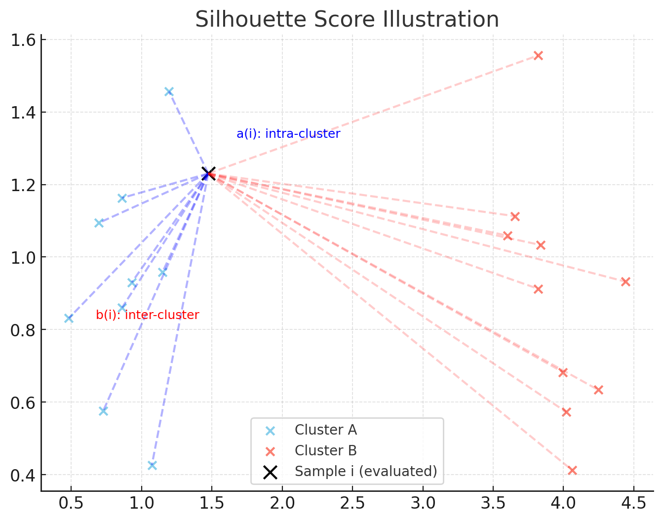
Consider 6 points in 2D, split into two clusters:

Cluster 0: (0,0), (0,1), (1,0)

Cluster 1: (5,5), (5,6), (6,5)

For point (0,0) in Cluster 0:

Computing a(0): Average distance to the other points in Cluster 0:

• Distance to (0,1) = 1.0
• Distance to (1,0) = 1.0
• a(0) = (1.0 + 1.0) / 2 = 1.0

Computing b(0): Average distance to all points in Cluster 1:

• Distance to (5,5) = \sqrt{50} \approx 7.07
• Distance to (5,6) = \sqrt{61} \approx 7.81
• Distance to (6,5) = \sqrt{61} \approx 7.81
• b(0) = (7.07 + 7.81 + 7.81) / 3 \approx 7.56

Since there are only 2 clusters, this is the only candidate for b.

Silhouette: s(0) = (7.56 - 1.0) / \max(1.0, 7.56) = 6.56 / 7.56 \approx 0.87

This point is well-clustered: it is much closer to its own cluster than to the other.

Repeating for all 6 points and averaging gives the overall silhouette score of approximately 0.79.

Why "Nearest" Cluster for b(i)?

The definition of b(i) uses the minimum average distance across all other clusters, not the average across all other clusters. This is deliberate.

If a point is far from most clusters but close to one neighboring cluster, it is in a precarious position. The worst-case neighbor is what matters for evaluating whether the point might be misclassified. Taking the minimum captures this: it identifies the cluster that most threatens the current assignment.

The cluster that achieves the minimum for b(i) is called the neighboring cluster of point i. If s(i) is negative, the neighboring cluster is where the point would likely be better assigned.

Using Silhouette Scores to Choose K

One of the most common uses of the silhouette score is selecting the number of clusters K for algorithms like K-Means.

The procedure:

1. Run the clustering algorithm for each candidate value of K (e.g., K = 2, 3, 4, \ldots, 10).
2. Compute the overall silhouette score for each K.
3. Choose the K that gives the highest silhouette score.

This is sometimes called the silhouette method for choosing K, and it is an alternative to the elbow method (which uses within-cluster sum of squares). The silhouette method has the advantage of producing a clearly defined optimum rather than a subjective "elbow."

However, the silhouette score tends to favor convex, similarly-sized clusters. For irregularly shaped or highly imbalanced clusters, it may not select the most meaningful K.

Silhouette Plots

Beyond the single overall score, silhouette plots visualize the silhouette value of every individual point, grouped by cluster. Each cluster forms a horizontal "blade" shape:

• The width of the blade is the silhouette value of each point.
• Points are sorted by silhouette value within each cluster.
• A vertical dashed line shows the overall average.

A good clustering produces blades that are roughly the same width (consistent cluster quality) and that extend well past the average line. If one cluster's blade is much narrower or has many negative values, that cluster is problematic.

Silhouette plots reveal issues that the single average score hides: a mediocre overall score might come from one excellent cluster and one terrible cluster, or from all clusters being equally mediocre.

Limitations of the Silhouette Score

Assumes convex clusters: The silhouette score uses average distances, which implicitly assumes clusters are roughly globular (convex). For non-convex clusters (e.g., crescent-shaped, ring-shaped), a point can be close to the wrong cluster in Euclidean distance even though it clearly belongs to its own cluster by shape. In these cases, the silhouette score can give misleadingly low values.

Sensitive to cluster density imbalance: If one cluster is very dense and another is very sparse, points in the sparse cluster will have large a(i) values and may receive low silhouette scores even if they are correctly clustered.

Computational cost: Computing all pairwise distances has O(N^2) time and space complexity. For very large datasets (millions of points), this becomes impractical. Approximations or sampling-based approaches are needed.

Only evaluates relative quality: A silhouette score of 0.6 does not mean the clustering is "good" in an absolute sense. It means points are, on average, closer to their own cluster than to the nearest other cluster by a moderate margin. Whether that is acceptable depends on the application.

Comparison with Other Clustering Metrics

Davies-Bouldin Index: Measures the average similarity between each cluster and its most similar cluster. Lower is better. Like the silhouette score, it is an internal metric that does not need ground truth. It is cheaper to compute (uses cluster centroids rather than all pairwise distances) but less informative at the individual-point level.

Calinski-Harabasz Index (Variance Ratio Criterion): The ratio of between-cluster dispersion to within-cluster dispersion. Higher is better. It is fast to compute but strongly biased toward convex clusters and sensitive to the number of clusters.

Adjusted Rand Index / Normalized Mutual Information: These are external metrics that require ground-truth labels. They measure how well the clustering agrees with the known labels. Useful for evaluation in research settings but not applicable when true labels are unknown.

The silhouette score strikes a balance: it provides per-point diagnostics (not just a single number), works without ground truth, and has an intuitive interpretation. Its main trade-off is computational cost.

Where the Silhouette Score Shows Up

Customer segmentation: After clustering customers by purchase behavior, the silhouette score helps determine whether the segments are meaningful or if the boundaries are arbitrary.

Image segmentation: Evaluating whether pixel clusters (regions) in an image are well-defined, particularly when comparing different segmentation algorithms.

Document clustering: Measuring whether groups of documents (clustered by topic) are coherent, helping choose the right number of topics for unsupervised topic modeling.

Bioinformatics: Evaluating gene expression clusters or protein structure groups, where ground-truth labels are often unavailable and the quality of groupings directly affects downstream analysis.

Examples

Hints

1. X[:, None, :] - X[None, :, :] forms every pairwise displacement.
2. A boolean matrix from labels[:, None] == labels[None, :] identifies same-cluster pairs.
3. Set each point's own-cluster column to infinity before taking the nearest other-cluster mean.

Requirements

• Compute pairwise Euclidean distances with NumPy broadcasting
• Support two or more clusters
• Avoid nested Python loops over pairs of samples
• Return the mean score as a Python float

Constraints

• X has shape (N,D) and labels has length N
• 2 \leq N \leq 500
• Every cluster contains at least two points
• Use NumPy only

Starter Code

import numpy as np

def silhouette_score(X: list, labels: list[int]) -> float:
    """
    Returns the mean Silhouette Score as a Python float.
    """
    # Write code here
    pass

Test Cases